Quantum Theory in Solids
Band Theory
In solid-state physics, the electronic band structure (or simply band structure) of a solid describes the range of energies that an electron within the solid may have (called energy bands, allowed bands, or simply bands) and ranges of energy that it may not have (called band gaps or forbidden bands).
Band theory derives these bands and band gaps by examining the allowed quantum mechanical wave functions for an electron in a large, periodic lattice of atoms or molecules. Band theory has been successfully used to explain many physical properties of solids, such as electrical resistivity and optical absorption, and forms the foundation of the understanding of all solid-state devices (transistors, solar cells, etc.).
The electrons of a single, isolated atom occupy atomic orbitals each of which has a discrete energy level. When two or more atoms join together to form into a molecule, their atomic orbitals overlap. The Pauli exclusion principle dictates that no two electrons can have the same quantum numbers in a molecule. So if two identical atoms combine to form a diatomic molecule, each atomic orbital splits into two molecular orbitals of different energy, allowing the electrons in the former atomic orbitals to occupy the new orbital structure without any having the same energy.
Similarly if a large number N of identical atoms come together to form a solid, such as a crystal lattice, the atoms' atomic orbitals overlap. Since the Pauli exclusion principle dictates that no two electrons in the solid have the same quantum numbers, each atomic orbital splits into N discrete molecular orbitals, each with a different energy. Since the number of atoms in a macroscopic piece of solid is a very large number (N~1022) the number of orbitals is very large and thus they are very closely spaced in energy (of the order of 10−22 eV). The energy of adjacent levels is so close together that they can be considered as a continuum, an energy band.
This formation of bands is mostly a feature of the outermost electrons (valence electrons) in the atom, which are the ones involved in chemical bonding and electrical conductivity. The inner electron orbitals do not overlap to a significant degree, so their bands are very narrow.
Band gaps are essentially leftover ranges of energy not covered by any band, a result of the finite widths of the energy bands. The bands have different widths, with the widths depending upon the degree of overlap in the atomic orbitals from which they arise. Two adjacent bands may simply not be wide enough to fully cover the range of energy. For example, the bands associated with core orbitals (such as 1s electrons) are extremely narrow due to the small overlap between adjacent atoms. As a result, there tend to be large band gaps between the core bands. Higher bands involve comparatively larger orbitals with more overlap, becoming progressively wider at higher energies so that there are no band gaps at higher energies.
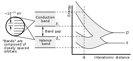
Showing how electronic band structure comes about by the hypothetical example of a large number of carbon atoms being brought together to form a diamond crystal. The graph (right) shows the energy levels as a function of the spacing between atoms. When the atoms are far apart (right side of graph) each atom has valence atomic orbitals p and s which have the same energy. However when the atoms come closer together their orbitals begin to overlap. Due to the Pauli Exclusion Principle each atomic orbital splits into N molecular orbitals each with a different energy, where N is the number of atoms in the crystal. Since N is such a large number, adjacent orbitals are extremely close together in energy so the orbitals can be considered a continuous energy band. a is the atomic spacing in an actual crystal of diamond. At that spacing the orbitals form two bands, called the valence and conduction bands, with a 5.5 eV band gap between them.
Assumptions and limits of band structure theory
Band theory is only an approximation to the quantum state of a solid, which applies to solids consisting of many identical atoms or molecules bonded together. These are the assumptions necessary for band theory to be valid:
- Infinite-size system: For the bands to be continuous, the piece of material must consist of a large number of atoms. Since a macroscopic piece of material contains on the order of 1022 atoms, this is not a serious restriction; band theory even applies to microscopic-sized transistors in integrated circuits. With modifications, the concept of band structure can also be extended to systems which are only "large" along some dimensions, such as two-dimensional electron systems.
- Homogeneous system: Band structure is an intrinsic property of a material, which assumes that the material is homogeneous. Practically, this means that the chemical makeup of the material must be uniform throughout the piece.
- Non-interactivity: The band structure describes "single electron states". The existence of these states assumes that the electrons travel in a static potential without dynamically interacting with lattice vibrations, other electrons, photons, etc.
The above assumptions are broken in a number of important practical situations, ad the use of band structure requires one to keep a close check on the limitations of band theory:
- Inhomogeneities and interfaces: Near surfaces, junctions, and other inhomogeneities, the bulk band structure is disrupted. Not only are there local small-scale disruptions (e.g., surface states or dopant states inside the band gap), but also local charge imbalances. These charge imbalances have electrostatic effects that extend deeply into semiconductors, insulators, and the vacuum (see doping, band bending).
- Along the same lines, most electronic effects (capacitance, electrical conductance, electric-field screening) involve the physics of electrons passing through surfaces and/or near interfaces. The full description of these effects, in a band structure picture, requires at least a rudimentary model of electron-electron interactions (see space charge, band bending).
- Small systems: For systems which are small along every dimension (e.g., a small molecule or a quantum dot), there is no continuous band structure. The crossover between small and large dimensions is the realm of mesoscopic physics.
- Strongly correlated materials (for example, Mott insulators) simply cannot be understood in terms of single-electron states. The electronic band structures of these materials are poorly defined (or at least, not uniquely defined) and may not provide useful information about their physical state.
Crystalline symmetry and wavevectors
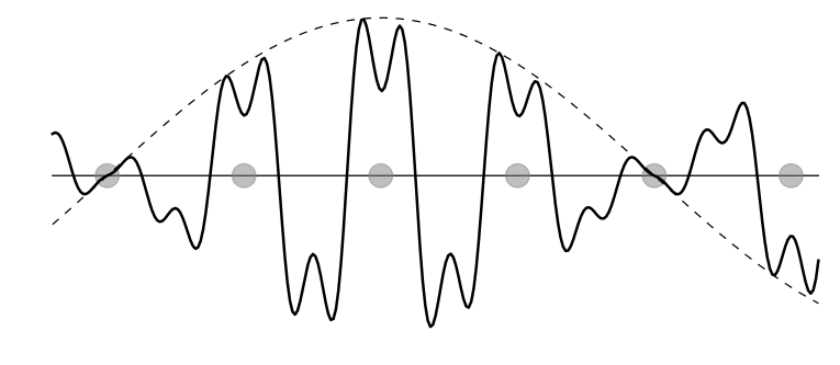
A Bloch wave (also called Bloch state or Bloch function or Bloch wavefunction), named after Swiss physicist Felix Bloch, is a type of wavefunction for a particle in a periodically-repeating environment, most commonly an electron in a crystal. A wavefunction ψ is a Bloch wave if it has the form:
Ψ(r) = eik.ru(r)
where r is position, ψ is the Bloch wave, u is a periodic function with the same periodicity as the crystal, k is a vector of real numbers called the crystal wave vector, e is Euler's number, and i is the imaginary unit. In other words, if we multiply a plane wave by a periodic function, we get a Bloch wave.
Bloch waves are important because of Bloch's theorem, which states that the energy eigenstates for an electron in a crystal can be written as Bloch waves. (More precisely, it states that the electron wave functions in a crystal have a basis consisting entirely of Bloch wave energy eigenstates.) This fact underlies the concept of electronic band structures.
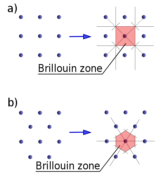
The first Brillouin zone is a uniquely defined primitive cell in reciprocal space. In the same way the Bravais lattice is divided up into Wigner–Seitz cells in the real lattice, the reciprocal lattice is broken up into Brillouin zones. The boundaries of this cell are given by planes related to points on the reciprocal lattice. The importance of the Brillouin zone stems from the Bloch wave description of waves in a periodic medium, in which it is found that the solutions can be completely characterized by their behavior in a single Brillouin zone.
The first Brillouin zone is the locus of points in reciprocal space that are closer to the origin of the reciprocal lattice than they are to any other reciprocal lattice points (see the derivation of the Wigner-Seitz cell). Another definition is as the set of points in k-space that can be reached from the origin without crossing any Bragg plane. Equivalently, this is the Voronoi cell around the origin of the reciprocal lattice.
There are also second, third, etc., Brillouin zones, corresponding to a sequence of disjoint regions (all with the same volume) at increasing distances from the origin, but these are used less frequently. As a result, the first Brillouin zone is often called simply the Brillouin zone. (In general, the n-th Brillouin zone consists of the set of points that can be reached from the origin by crossing exactly n − 1 distinct Bragg planes.)
A related concept is that of the irreducible Brillouin zone, which is the first Brillouin zone reduced by all of the symmetries in the point group of the lattice (point group of the crystal).
These Bloch wave energy eigenstates are written with subscripts as ψn k, where n is a discrete index, called the band index, which is present because there are many different Bloch waves with the same k (each has a different periodic component u). Within a band (i.e., for fixed n), ψnk varies continuously with k, as does its energy. Also, for any reciprocal lattice vector K, ψnk = ψn,(k+K). Therefore, all distinct Bloch waves occur for k-values within the first Brillouin zone of the reciprocal lattice.
Band structure calculations take advantage of the periodic nature of a crystal lattice, exploiting its symmetry. The single-electron Schrödinger equation is solved for an electron in a lattice-periodic potential, giving Bloch waves as solutions. For each value of k, there are multiple solutions to the Schrödinger equation labelled by n, the band index, which simply numbers the energy bands. Each of these energy levels evolves smoothly with changes in k, forming a smooth band of states. For each band we can define a function En(k), which is the dispersion relation for electrons in that band.
The wavevector takes on any value inside the Brillouin zone, which is a polyhedron in wavevector space that is related to the crystal's lattice. Wavevectors outside the Brillouin zone simply correspond to states that are physically identical to those states within the Brillouin zone. Special high symmetry points/lines in the Brillouin zone are assigned labels like Γ, Δ, Λ, Σ.
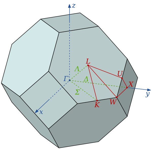
It is difficult to visualize the shape of a band as a function of wavevector, as it would require a plot in four-dimensional space, E vs. kx, ky, kz. In scientific literature it is common to see band structure plots which show the values of En(k) for values of k along straight lines connecting symmetry points, often labelled Δ, Λ, Σ, or [100], [111], and [110], respectively. Another method for visualizing band structure is to plot a constant-energy isosurface in wavevector space, showing all of the states with energy equal to a particular value. The isosurface of states with energy equal to the Fermi level is known as the Fermi surface.
Energy band gaps can be classified using the wavevectors of the states surrounding the band gap:
- Direct band gap: the lowest-energy state above the band gap has the same k as the highest-energy state beneath the band gap.
- Indirect band gap: the closest states above and beneath the band gap do not have the same k value.
Density of states
density of states (DOS) of a system describes the number of states per an interval of energy at each energy level available to be occupied. It is mathematically represented by a density distribution and it is generally an average over the space and time domains of the various states occupied by the system. A high DOS at a specific energy level means that there are many states available for occupation. A DOS of zero means that no states can be occupied at that energy level. The DOS is usually represented by one of the symbols g, ρ, D, n, or N. Generally, the density of the states of matter is continuous. In isolated systems however, like atoms or molecules in the gas phase, the density distribution is discrete like a spectral density.
Local variations, most often due to distortions of the original system, are often called local density of states (LDOS). If the DOS of an undisturbed system is zero, the LDOS can locally be non-zero due to the presence of a local potential.
The density of states function g(E) is defined as the number of electronic states per unit volume, per unit energy, for electron energies near E.
The density of states function is important for calculations of effects based on band theory. In Fermi's Golden Rule, a calculation for the rate of optical absorption, it provides both the number of excitable electrons and the number of final states for an electron. It appears in calculations of electrical conductivity where it provides the number of mobile states, and in computing electron scattering rates where it provides the number of final states after scattering.
For energies inside a band gap, g(E) = 0.
Filling of bands
The Fermi level chemical potential for electrons (or electrochemical potential for electrons), usually denoted by µ or EF, of a body is a thermodynamic quantity, whose significance is the thermodynamic work required to add one electron to the body (not counting the work required to remove the electron from wherever it came from). A precise understanding of the Fermi level—how it relates to electronic band structure in determining electronic properties, how it relates to the voltage and flow of charge in an electronic circuit—is essential to an understanding of solid-state physics. In band structure theory, used in solid state physics to analyze the energy levels in a solid, the Fermi level can be considered to be a hypothetical energy level of an electron, such that at thermodynamic equilibrium this energy level would have a 50% probability of being occupied at any given time
At thermodynamic equilibrium, the likelihood of a state of energy E being filled with an electron is given by the Fermi–Dirac distribution, a thermodynamic distribution that takes into account the Pauli exclusion principle:
f(E) = 1/[1 + e(E - µ)/kBT]
where: kBT is the product of Boltzmann's constant and temperature, and µ is the total chemical potential of electrons, or Fermi level (in semiconductor physics, this quantity is more often denoted EF). The Fermi level of a solid is directly related to the voltage on that solid, as measured with a voltmeter. Conventionally, in band structure plots the Fermi level is taken to be the zero of energy (an arbitrary choice).
The density of electrons in the material is simply the integral of the Fermi–Dirac distribution times the density of states:
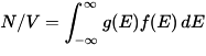
Although there are an infinite number of bands and thus an infinite number of states, there are only a finite number of electrons to place in these bands. The preferred value for the number of electrons is a consequence of electrostatics: even though the surface of a material can be charged, the internal bulk of a material prefers to be charge neutral. The condition of charge neutrality means that N/V must match the density of protons in the material. For this to occur, the material electrostatically adjusts itself, shifting its band structure up or down in energy (thereby shifting g(E)), until it is at the correct equilibrium with respect to the Fermi level.

Filling of the electronic states in various types of materials at equilibrium. Here, height is energy while width is the density of available states for a certain energy in the material listed. The shade follows the Fermi–Dirac distribution (black = all states filled, white = no state filled). In metals and semimetals the Fermi level EF lies inside at least one band. In insulators and semiconductors the Fermi level is inside a band gap; however, in semiconductors the bands are near enough to the Fermi level to be thermally populated with electrons or holes.
Names of bands near the Fermi level (conduction band, valence band)
A solid has an infinite number of allowed bands, just as an atom has infinitely many energy levels. However, most of the bands simply have too high energy, and are usually disregarded under ordinary circumstances. Conversely, there are very low energy bands associated with the core orbitals (such as 1s electrons). These low-energy core bands are also usually disregarded since they remain filled with electrons at all times, and are therefore inert. Likewise, materials have several band gaps throughout their band structure.
The most important bands and band gaps—those relevant for electronics and optoelectronics—are those with energies near the Fermi level. The bands and band gaps near the Fermi level are given special names, depending on the material:
In a semiconductor or band insulator, the Fermi level is surrounded by a band gap, referred to as the band gap (to distinguish it from the other band gaps in the band structure). The closest band above the band gap is called the conduction band, and the closest band beneath the band gap is called the valence band. The name "valence band" was coined by analogy to chemistry, since in semiconductors (and insulators) the valence band is built out of the valence orbitals.
In a metal or semimetal, the Fermi level is inside of one or more allowed bands. In semimetals the bands are usually referred to as "conduction band" or "valence band" depending on whether the charge transport is more electron-like or hole-like, by analogy to semiconductors. In many metals, however, the bands are neither electron-like nor hole-like, and often just called "valence band" as they are made of valence orbitals. The band gaps in a metal's band structure are not important for low energy physics, since they are too far from the Fermi level.
Resume of Band Theory
Band theory, in solid-state physics, theoretical model describing the states of electrons, in solid materials, that can have values of energy only within certain specific ranges. The behaviour of an electron in a solid (and hence its energy) is related to the behaviour of all other particles around it. This is in direct contrast to the behaviour of an electron in free space where it may have any specified energy. The ranges of allowed energies of electrons in a solid are called allowed bands. Certain ranges of energies between two such allowed bands are called forbidden bands—i.e., electrons within the solid may not possess these energies. The band theory accounts for many of the electrical and thermal properties of solids and forms the basis of the technology of solid-state electronics.
The band of energies permitted in a solid is related to the discrete allowed energies—the energy levels—of single, isolated atoms. When the atoms are brought together to form a solid, these discrete energy levels become perturbed through quantum mechanical effects, and the many electrons in the collection of individual atoms occupy a band of levels in the solid called the valence band. Empty states in each single atom also broaden into a band of levels that is normally empty, called the conduction band. Just as electrons at one energy level in an individual atom may transfer to another empty energy level, so electrons in the solid may transfer from one energy level in a given band to another in the same band or in another band, often crossing an intervening gap of forbidden energies. Studies of such changes of energy in solids interacting with photons of light, energetic electrons, X-rays, and the like confirm the general validity of the band theory and provide detailed information about allowed and forbidden energies.
A variety of ranges of allowed and forbidden bands is found in pure elements, alloys, and compounds. Three distinct groups are usually described: metals, insulators, and semiconductors. In metals, forbidden bands do not occur in the energy range of the most energetic (outermost) electrons. Accordingly, metals are good electrical conductors. Insulators have wide forbidden energy gaps that can be crossed only by an electron having an energy of several electron volts. Because electrons cannot move freely in the presence of an applied voltage, insulators are poor conductors. Semiconductors have relatively narrow forbidden gaps—which can be crossed by an electron having an energy of roughly one electron volt—and so are intermediate conductors.
Understanding Magnetic Phenomena
Magnetic materials were then classified as dia, para and ferromagnetics. Theoretical understanding of these phenomena required inputs from two sources, (1) electromagnetism and (2) atomic theory. Electromagnetism, that unified electricity and magnetism, showed that moving charges produce magnetic fields and moving magnets produce emf’s in conductors. The fact that electrons (discovered in 1897) reside in atoms directed attention to the question whether magnetic properties of materials had a relation with the motions of electrons in atoms.
The theory of diamagnetism was successfully explained to be due to the Lorentz force
F = e[E + (1/c)v x H]
on an orbiting electron when a magnetic field H is applied. Here v is the velocity of the electron and 'e' the electronic charge (Langevin 1905, Pauli 1920). This changes the electric current in the electron orbit, in a way that gives an induced magnetization
Minduced = -(Ne2/6mc2)z(r2)H
where √(r2) is the typical radius of the electron orbit in the atom, with the negative sign implying that the induced effect opposes the external applied one, 'N' is the number of atoms per unit volume and 'z' is the atomic number, i.e. the number of electrons per atom and 'm,' is the electronic mass. Diamagnetism is a universal phenomenon present in all substances, but being a feeble effect, may be subsumed by paramagnetism if paramagnetism is present. Paramagnetism of materials, as was rightly concluded, is related to the fact that atoms or molecules can have permanent dipole moments. These permanent dipole moments arise due to the fact that every orbiting electron is a current loop, that acts as a tiny magnetic shell, giving by Ampere's law, a magnetic moment
μ = μB∑(Li + 2Si)
Here, μB = (eh/4πmc) is called the Bohr magneton, Li and Si are the quantum numbers of orbital and spin angular momenta respectively, 'h' is the Planck constant and the summation in μ equation is evaluated for all the 'z' electrons in the atom. Whether an atom or a molecule has a permanent dipole moment or not is decided by whether the sum in equation above is non zero or not - a scheme that is documented in several text books. Physicists, however, failed to understand ferromagnetism from an atomic basis. It was Heisenberg's work in the late 1920's that filled this void. To accomplish this, quantum mechanics had to be discovered first. This was done mainly to understand atomic spectra. It was indeed in the fitness of things that the quantum dynamics of the electron left an imprint on another area, namely magnetism, which too had to do with the magnetic effects of electron dynamics. To understand this development we take a little digression into the phenomenology of ferromagnetism and into the area of electron bonding, which to most of the classical physicists were unconnected phenomena. It was Heisenberg, who saw the connection and established it in two seminal papers, written in 1926 and 1928.
Ferromagnetism
It was found that certain substances like iron, cobalt, nickel, etc., when cooled below a certain temperature Tc (called the critical temperature) developed a spontaneous magnetization, even in the absence of an external magnetic field. The temperature variation of the magnetic susceptibility above the critical temperature was found to follow the Curie-Weiss law Xferro = C /(T - Tc), whereas an ordinary paramagnet shows the Curie law: X = C/T It was Weiss, in 1907, who correctly understood that this dependence was due to an internal magnetic field Hint., called the molecular magnetic field. This was such that if an external magnetic field H is applied, then every atom in the substance finds itself in an effective magnetic field
Heff = H + Hint. = H + αM
Here M, the magnetization, is given by
M = ∑μj
where the summation is over all atoms, present in a unit volume and α > 0, is a parameter characteristic of the substance. This internal field Hint. = αM is seen to play an ordering effect as can be seen below. If we bring a dipole from outside and place it in the internal field, the di pole will be aligned in the direction of this internal field, i.e., in the direction of the magnetization itself, giving rise to a spontaneous ordering, i.e., yield a ferromagnetic state. This ordering effect is indeed destroyed by the randomizing energy kBT arising due to thermal effects, trying to flip the dipole away from this ordered state. Calculations of the magnetization show that (if the dipoles can align only in two directions ↑ and ↓),
M(H) = Nμ tanh(μ[H + αM]/kBT)
In the absence of the external magnetic field (H = 0), the magnetization follows
M = Nμ tanh(μαM/kBT)
This shows that a non zero solution for M i.e. a spontaneous magnetization is possible only if T < Tc = Nμ2α/kB. The susceptibility is seen to follow, for high temperatures,
Xferro ≡ ∂M(H)/∂H ≈ Nμ2/kB)/(T – Tc)
obeying the experimentally observed Curie-Weiss law, while the spontaneous magnetization follows M(H = 0, T) ∝ √(Tc - T), for T ≤ Tc. From the fact that the transition temperature Tc follows kBTc = Nμ2α, it is clear that the ordered ferromagnetic state can occur when the diminution of energy, Nμ2α per dipole, due to ferromagnetic ordering exceeds the randomizing thermal energy kBT.
Ferromagnetic materials such as iron are characterized by the way in which their magnetic properties change dramatically at a particular critical temperature, called the Curie temperature. Below the Curie temperature a ferromagnetic material can carry a strong remanent magnetization, but above the Curie temperature, its ferromagnetic ordering is broken down by thermal energy and it behaves as a paramagnet.
The remanent magnetization of ferromagnetic materials results from the phenomenon of spontaneous magnetization — that is a magnetization which exists even in the absence of a magnetic field. Spontaneous magnetizations arise from the group- magnetic phenomenon of exchange interactions. In these interactions all elementary magnetic moments of neighboring electrons are aligned parallel with one another by quantum mechanical effects.
Another important property of ferromagnetic materials is that their net magnetic moment is much greater than that of paramagnetic and diamagnetic materials. This strong magnetic moment of ferromagnets arises because the magnetic exchange interactions between neighboring atoms are so powerful that they are able to align the ferromagnetic atomic moments despite the continual disturbance of thermal agitation.
Landau Diamagnetism
Diamagnetism is a fundamental magnetic property. It is extremely weak compared with other magnetic effects and so it tends to be swamped by all other types of magnetic behaviour. Diamagnetism arises from the interaction of an applied magnetic field with the orbital motion of electrons and it results in a very weak negative magnetisation. The magnetisation is lost as soon as the magnetic field is removed. Strong magnetic fields tend to repel diamagnetic materials. The spin magnetic moments of electrons do not con- tribute to the magnetisation of diamagnets as all the electron spin motions are paired and cancel each other out.
Diamagnetism is for all practical purposes independent of temperature. Many common natural minerals, such as quartz, feldspar, calcite and water, exhibit diamagnetic behaviour.
Paramagnetism
Paramagnetic behavior can occur when individual atoms, ions or molecules possess a permanent elementary magnetic dipole moment. Such magnetic dipoles tend to align themselves parallel with the direction of any applied field and to cause a weak positive magnetization. However, the magnetization of a paramagnet is lost once the field is removed because of thermal effects. In an applied field, para- magnetic materials behave in the opposite way to diamagnetic materials and tend to be attracted to regions of strong field. Many natural minerals, e.g. olivine, pyroxene, garnet, biotite, and carbonates of iron and manganese, are paramagnetic. The incompletely filled inner electron shells of Mn2+, Fe2+ and Fe3+ ions are generally responsible for the para- magnetic behavior of natural materials as they have unpaired electrons with free spin magnetic moments.
When a field is applied to a paramagnetic substance the spin magnetic moments tend to order and to orientate parallel to the applied field direction. How- ever, the magnetic energies involved are small and thermal agitation constantly attempts to break down the magnetic ordering. A balance is reached between these two competing processes of thermal randomizing and magnetic ordering. The magnetic moment which depends on this balance is thus a function of both the applied field and the absolute temperature. The magnetization of a paramagnetic substance is very weak compared with that of a ferromagnetic, but paramagnetic effects are in turn dominant over diamagnetic effects.
Ferrimagnetism and antiferromagnetism
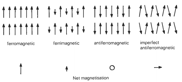
The main natural magnetic minerals we shall be dealing with are special variants of ferromagnets known as ferrimagnets and imperfect antiferromagnets. Ferrimagnetic and antiferromagnetic behavior in natural materials arises from ordering of the spin magnetic moments of electrons in the incompletely filled 3d shells of first transition series elements, particularly iron and manganese, by exchange forces.
Ferrimagnetism
Ferrimagnetism is outwardly very similar to ferromagnetism; indeed, it is very difficult to distinguish between the two properties even using magnetic measuring techniques. Ferrimagnetic materials carry a remanent magnetization below a critical temperature, termed the Curie or Néel temperature, and like ferromagnets they are paramagnetic above this temperature.
The magnetic behavior of ferrites (ferrimagnets) depends on their particular crystal structure. Ferrites are commonly iron oxides with a spinel (close-packed face-centred cubic) structure containing two types of magnetic sites which have antiparallel magnetic moments of different magnitudes. Therefore, the elementary magnetic moments of a ferrite are regularly ordered in an antiparallel sense, but the sum of the moments pointing in one direction exceeds that in the opposite direction leading to a net magnetization. The imbalance in lattice moments in ferrites may be due to different ionic populations on the two types of sites or to crystallographic dis- similarities between the two types of magnetic sites.
Ferrites have low electrical conductivities and have many industrial applications. For example, Mn and Zn ferrites are used in radiofrequency cores, while Mn mixture ferrites are used in computer memories. Magnetite is an example of a natural ferrite.
Antiferromagnetism
In antiferromagnetic materials there are again two magnetic sublattices which are antiparallel, but their magnetic moments are identical, and so the material exhibits zero bulk spontaneous magnetization. Antiferromagnetic ordering is also destroyed by thermal agitation at the Néel temperature. Modification of the basic antiferromagnetic arrangement can, however, lead to a net spontaneous magnetization. Two such imperfect antiferromagnetic forms are parasitic ferromagnetism which may result from heterogeneities due to impurities or lattice defects, and by spin canting, which arises from a slight modification of the true antiferromagnetic anti- parallelism. Spin canting is illustrated in figure below. The mineral hematite is an example of a natural crystal with an imperfect antiferromagnetic structure caused by spin canting.
Hysteresis
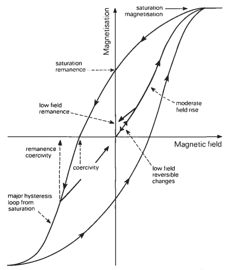
The magnetic state of an iron bar depends on both the magnetic field to which it is subjected and the history of the bar. The field dependence of magnetization can be described with the aid of Figure below which plots magnetization on the vertical axis against magnetic field on the horizontal axis. Starting with an unmagnetized piece of iron it is found that its magnetization increases slowly as a small field is applied and that if this field is removed the magnetization returns to zero. However, on applying a stronger field, beyond a certain critical field, it is found that an important change in magnetic behavior takes place. The magnetization is now no longer reversible in the straightforward way of the very low fields; instead, on removal of the field, a phenomenon referred to as hysteresis develops. In short, changes in magnetization associated with the removal of the field now differ from those that occurred during the preceding increase of the field, in such a way that the magnetization changes lag behind the field. Furthermore, it is found that on complete removal of the field, i.e. in zero field, the iron is no longer unmagnetized but has a remanent magnetization. At moderate fields magnetization rises sharply with increasing field and at still higher fields saturation of the magnetization sets in and the magnetization curve flattens out. A complete hysteresis loop is obtained by cycling the magnetic field from an extreme applied field in one direction to an extreme in the opposite direction and back again.
Many of the simple magnetic properties used in later chapters to characterize materials can be classed as hysteresis parameters and the interrelationships between these properties can be best understood in terms of hysteresis loops. Consider five of the most important hysteresis parameters. Saturation magnetization, Ms, is the magnetization induced in the presence of a large (> 1 T) magnetic field. Upon removal of this field the magnetization does not decrease completely to zero. The remaining magnetization is called the saturation remanent magnetization, Mps. By the application of a field, in the opposite direction to that first used, the induced magnetization can be reduced to zero. The reverse field which actually makes the magnetization zero, when measurement is made in the presence of the field, is called the saturation coercivity (B0)c. An even larger reverse field is needed to leave no remanent magnetization after its subsequent withdrawal. This reverse field is called the coercivity of remanence, (B0)cr. The gradient of the magnetization curve at the origin of figure below is the initial susceptibility, K.
Chemical Bonds
The dynamics of scientific progress is indeed one of cooperative phenomenon, where the seeds of the breakthrough in one field may be sown in another. So was the case with magnetism, where the fundamental mechanism for the origin of the co-operative field was being investigated in the field of spectroscopy, in trying to understand the origin of the chemical bond. The chemist had a dilemma ever since the discovery of the electron. The question was this: if every atom has an outer cloud of electrons, then how do atoms approach each other to form a chemical bond? The problem was first tried by Pauli (1926) in the context of the helium atom and by Heider and London (1927) for the hydrogen molecule.
The a hove works can be classified under spectroscopy and chemical bonding but it was Heisenberg who showed that the interaction between electrons, called the exchange energy was indeed the basis of the Weiss molecular field. It is here that some experimental results are in order. In most cases it is seen that: kBTc ≈ 10-14 erg. The dipole-dipole interaction between the atomic dipoles, kept at about 1 Angstrom (10-8 cm) away can contribute only an energy of the order of 10-16 ergs, hence a stronger agency is required to bring in the Weiss molecular field. Heisenberg correctly identified that the exchange energy, which is of electrostatic origin (with a typical energy 10-14 erg and not a dipole-dipole interaction) and is purely quantum mechanical in nature, lies at the core of what gives rise to the Weiss field.
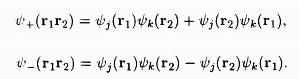
According to the Heitler-London theory, if there are two atoms, '1' and '2' each having a single electron, one can assun1e them to be in atomic states 'j' and 'k' the orbital wave functions for this two-electron system can be constructed from the linear combinations of the quantities Ψj(r1)Ψk(r2), Ψj(r2)Ψk(r1), where r1, r2 are the locations in space for the two electrons. The possible wave functions are
One must, in addition, consider the spin part of the wave function. The spin of any electron can point up ↑ or down ↓. The spin part of the two electron wave function can be

In the case S1, since both the spins are pointing in the same direction, the net spin is (s = 1/2 + 1/2 = 1) while in the case S0, since the two spins are Rointing in opposite directions, the net spin is (s = 1/2 - 1/2 = 0). The total number of possible states g = 2s + 1 gives the degeneracy of the respective states to be g0 = 1 and g1 = 3. Suppose we apply the external magnetic field in the z-direction, then for S0 the z components of the spin can be sz = 0, while for S1 they can be sz = 1,0, -1.
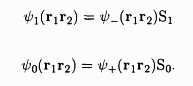
The total wave function of the two-electron system must combine both the orbital as well as the spin wave functions, and by the Pauli exclusion principle, should be such that if the two electrons are in the same state, the wave function must vanish identically. It is seen that this is possible only if the wave functions are:
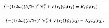
To find the energy eigenvalues of this two-electron system, one has to solve the Schrodinger equation

while V(r1), V(r2) are the potentials in the two atoms and the last term in the RHS of the equation of S0 describes the electrostatic Coulomb interaction between the two electrons. The atomic states 'j' and 'k' being those in the absence of the electron-electron Coulomb interaction, we have
Assunling the zeroth order wave functions to be Ψ1(r1, r2), Ψ0(r1, r2), given in wave function equation, one finds in the first order approximation, the energy eigenvalues of the singlet (suffix 0) and the triplet (suffix 1) states to be
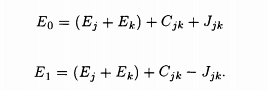
Here the terms Cjk and Jjk are given by the integrals
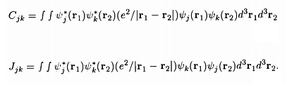
It is seen that Cjk is the Coulomb energy of interaction between the two electrons, since Ψj*(r1)Ψj(r1) gives the electron density at r1, and Ψk*(r2)Ψk(r2) gives the electron density at r2 The term Jjk is called the exchange integral (since Ψj*(r1) couples with Ψk(r1) while Ψk*(r2) couples with Ψj(r2)) and has no classical analogue.
An Introduction to the Concept of Band Structure.HyperPhysics - Bands in Solids
Multiferroic Materials Physics and Properties.SOLID STATE PHYSICS - Magnetic Properties of Solids.
REFERENCES
Encyclopaedia Britannica. Available in: https://www.britannica.com/science/band-theory. Access in: 13/10/2018.
Wikipedia. Available in: https://en.wikipedia.org/wiki/Electronic_band_structure. Access in: 13/10/2018.
Wikipedia. Available in: https://en.wikipedia.org/wiki/Bloch_wave. Access in: 13/10/2018.
Wikipedia. Available in: https://en.wikipedia.org/wiki/Brillouin_zone. Access in: 13/10/2018.
Wikipedia. Available in: https://en.wikipedia.org/wiki/Density_of_states. Access in: 13/10/2018.
Wikipedia. Available in: https://en.wikipedia.org/wiki/Fermi_level. Access in: 13/10/2018.
University of Edinburgh. Available in: https://www.geos.ed.ac.uk/homes/thompson/envmag/Envmag_2_3.pdf. Access in: 13/10/2018.
Indian Academy of Sciences. Available in: https://www.ias.ac.in/article/fulltext/reso/009/08/0057-0066. Access in: 13/10/2018.
WHITE, Robert M. Springer series in solid-state sciences - Quantum theory of magnetism: Magnetic properties of materials. 3th edition, Sringer, 2007. p. 85-106.


0 comments
Sign in or create a free account