The Quantum Electrodynamics

Quantum electrodynamics (QED) is the relativistic quantum field theory of electrodynamics. In essence, it describes how light and matter interact and is the first theory where full agreement between quantum mechanics and special relativity is achieved. QED mathematically describes all phenomena involving electrically charged particles interacting by means of exchange of photons and represents the quantum counterpart of classical electromagnetism giving a complete account of matter and light interaction.

In technical terms, QED can be described as a perturbation theory of the electromagnetic quantum vacuum. Richard Feynman called it "the jewel of physics" for its extremely accurate predictions of quantities like the anomalous magnetic moment of the electron and the Lamb shift of the energy levels of hydrogen.

Difficulties with the theory increased through the end of the 1940s. Improvements in microwave technology made it possible to take more precise measurements of the shift of the levels of a hydrogen atom, now known as the Lamb shift and magnetic moment of the electron. These experiments exposed discrepancies which the theory was unable to explain.

A first indication of a possible way out was given by Hans Bethe in 1947, after attending the Shelter Island Conference. While he was traveling by train from the conference to Schenectady he made the first non-relativistic computation of the shift of the lines of the hydrogen atom as measured by Lamb and Retherford. Despite the limitations of the computation, agreement was excellent. The idea was simply to attach infinities to corrections of mass and charge that were actually fixed to a finite value by experiments. In this way, the infinities get absorbed in those constants and yield a finite result in good agreement with experiments. This procedure was named renormalization.

Based on Bethe's intuition and fundamental papers on the subject by Shinichiro Tomonaga, Julian Schwinger, Richard Feynman and Freeman Dyson, it was finally possible to get fully covariant formulations that were finite at any order in a perturbation series of quantum electrodynamics. Shin'ichirō Tomonaga, Julian Schwinger and Richard Feynman were jointly awarded with a Nobel prize in physics in 1965 for their work in this area.

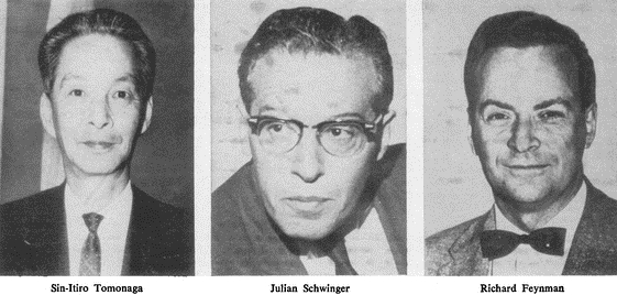
Their contributions, and those of Freeman Dyson, were about covariant and gauge invariant formulations of quantum electrodynamics that allow computations of observables at any order of perturbation theory. Feynman's mathematical technique, based on his diagrams, initially seemed very different from the field-theoretic, operator-based approach of Schwinger and Tomonaga, but Freeman Dyson later showed that the two approaches were equivalent. Renormalization, the need to attach a physical meaning at certain divergences appearing in the theory through integrals, has subsequently become one of the fundamental aspects of quantum field theory and has come to be seen as a criterion for a theory's general acceptability. Even though renormalization works very well in practice, Feynman was never entirely comfortable with its mathematical validity, even referring to renormalization as a "shell game" and "hocus pocus".

QED has served as the model and template for all subsequent quantum field theories. One such subsequent theory is quantum chromodynamics, which began in the early 1960s and attained its present form in the 1970s work by H. David Politzer, Sidney Coleman, David Gross and Frank Wilczek. Building on the pioneering work of Schwinger, Gerald Guralnik, Dick Hagen, and Tom Kibble, Peter Higgs, Jeffrey Goldstone, and others, Sheldon Glashow, Steven Weinberg and Abdus Salam independently showed how the weak nuclear force and quantum electrodynamics could be merged into a single electroweak force.

Near the end of his life, Richard P. Feynman gave a series of lectures on QED intended for the lay public. These lectures were transcribed and published as Feynman (1985), QED: The strange theory of light and matter, a classic non-mathematical exposition of QED from the point of view articulated below.

The key components of Feynman's presentation of QED are three basic actions.

• A photon goes from one place and time to another place and time.
  
• An electron goes from one place and time to another place and time.
  
• An electron emits or absorbs a photon at a certain place and time.
  

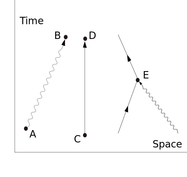
These actions are represented in the form of visual shorthand by the three basic elements of Feynman diagrams: a wavy line for the photon, a straight line for the electron and a junction of two straight lines and a wavy one for a vertex representing emission or absorption of a photon by an electron. These can all be seen in the adjacent diagram.

As well as the visual shorthand for the actions Feynman introduces another kind of shorthand for the numerical quantities called probability amplitudes. The probability is the square of the absolute value of total probability amplitude,

Probability = |f(amplitude)|²

If a photon moves from one place and time A to another place and time B, the associated quantity is written in Feynman's shorthand as P(A to B). The similar quantity for an electron moving from C to D is written E(C to D). The quantity that tells us about the probability amplitude for the emission or absorption of a photon he calls j. This is related to, but not the same as, the measured electron charge e.

QED is based on the assumption that complex interactions of many electrons and photons can be represented by fitting together a suitable collection of the above three building blocks and then using the probability amplitudes to calculate the probability of any such complex interaction. It turns out that the basic idea of QED can be communicated while assuming that the square of the total of the probability amplitudes mentioned above (P(A to B), E(C to D) and j) acts just like our everyday probability (a simplification made in Feynman's book). Later on, this will be corrected to include specifically quantum-style mathematics, following Feynman.

The basic rules of probability amplitudes that will be used are:

• If an event can happen in a variety of different ways, then its probability amplitude is the sum of the probability amplitudes of the possible ways.
  
• If a process involves a number of independent sub-processes, then its probability amplitude is the product of the component probability amplitudes.
  

Basic constructions

Suppose, we start with one electron at a certain place and time (this place and time being given the arbitrary label A) and a photon at another place and time (given the label B). A typical question from a physical standpoint is: "What is the probability of finding an electron at C (another place and a later time) and a photon at D (yet another place and time)?". The simplest process to achieve this end is for the electron to move from A to C (an elementary action) and for the photon to move from B to D (another elementary action). From a knowledge of the probability amplitudes of each of these sub-processes – E(A to C) and P(B to D) – we would expect to calculate the probability amplitude of both happening together by multiplying them, using rule b) above. This gives a simple estimated overall probability amplitude, which is squared to give an estimated probability.

But there are other ways in which the end result could come about. The electron might move to a place and time E, where it absorbs the photon; then move on before emitting another photon at F; then move on to C, where it is detected, while the new photon moves on to D. The probability of this complex process can again be calculated by knowing the probability amplitudes of each of the individual actions: three electron actions, two photon actions and two vertexes – one emission and one absorption. We would expect to find the total probability amplitude by multiplying the probability amplitudes of each of the actions, for any chosen positions of E and F. We then, using rule a) above, have to add up all these probability amplitudes for all the alternatives for E and F. (This is not elementary in practice and involves integration.) But there is another possibility, which is that the electron first moves to G, where it emits a photon, which goes on to D, while the electron moves on to H, where it absorbs the first photon, before moving on to C. Again, we can calculate the probability amplitude of these possibilities (for all points G and H). We then have a better estimation for the total probability amplitude by adding the probability amplitudes of these two possibilities to our original simple estimate. Incidentally, the name given to this process of a photon interacting with an electron in this way is Compton scattering.

There is an infinite number of other intermediate processes in which more and more photons are absorbed and/or emitted. For each of these possibilities, there is a Feynman diagram describing it. This implies a complex computation for the resulting probability amplitudes, but provided it is the case that the more complicated the diagram, the less it contributes to the result, it is only a matter of time and effort to find as accurate an answer as one wants to the original question. This is the basic approach of QED. To calculate the probability of any interactive process between electrons and photons, it is a matter of first noting, with Feynman diagrams, all the possible ways in which the process can be constructed from the three basic elements. Each diagram involves some calculation involving definite rules to find the associated probability amplitude.

That basic scaffolding remains when one moves to a quantum description, but some conceptual changes are needed. One is that whereas we might expect in our everyday life that there would be some constraints on the points to which a particle can move, that is not true in full quantum electrodynamics. There is a possibility of an electron at A, or a photon at B, moving as a basic action to any other place and time in the universe. That includes places that could only be reached at speeds greater than that of light and also earlier times. (An electron moving backwards in time can be viewed as a positron moving forward in time).

Probability amplitudes

Quantum mechanics introduces an important change in the way probabilities are computed. Probabilities are still represented by the usual real numbers we use for probabilities in our everyday world, but probabilities are computed as the square of probability amplitudes, which are complex numbers.

Feynman avoids exposing the reader to the mathematics of complex numbers by using a simple but accurate representation of them as arrows on a piece of paper or screen. (These must not be confused with the arrows of Feynman diagrams, which are simplified representations in two dimensions of a relationship between points in three dimensions of space and one of time.) The amplitude arrows are fundamental to the description of the world given by quantum theory. They are related to our everyday ideas of probability by the simple rule that the probability of an event is the square of the length of the corresponding amplitude arrow. So, for a given process, if two probability amplitudes, v and w, are involved, the probability of the process will be given either by

P = |v + w|² or P = |vw|²

The rules as regards adding or multiplying, however, are the same as above. But where you would expect to add or multiply probabilities, instead you add or multiply probability amplitudes that now are complex numbers.

Addition and multiplication are common operations in the theory of complex numbers and are given in the figures. The sum is found as follows. Let the start of the second arrow be at the end of the first. The sum is then a third arrow that goes directly from the beginning of the first to the end of the second. The product of two arrows is an arrow whose length is the product of the two lengths. The direction of the product is found by adding the angles that each of the two have been turned through relative to a reference direction: that gives the angle that the product is turned relative to the reference direction.

That change, from probabilities to probability amplitudes, complicates the mathematics without changing the basic approach. But that change is still not quite enough because it fails to take into account the fact that both photons and electrons can be polarized, which is to say that their orientations in space and time have to be taken into account. Therefore, P(A to B) consists of 16 complex numbers, or probability amplitude arrows: There are also some minor changes to do with the quantity j, which may have to be rotated by a multiple of 90° for some polarizations, which is only of interest for the detailed bookkeeping.

Associated with the fact that the electron can be polarized is another small necessary detail, which is connected with the fact that an electron is a fermion and obeys Fermi–Dirac statistics. The basic rule is that if we have the probability amplitude for a given complex process involving more than one electron, then when we include (as we always must) the complementary Feynman diagram in which we exchange two electron events, the resulting amplitude is the reverse – the negative – of the first. The simplest case would be two electrons starting at A and B ending at C and D. The amplitude would be calculated as the "difference", E(A to D) × E(B to C) − E(A to C) × E(B to D), where we would expect, from our everyday idea of probabilities, that it would be a sum.

Mass renormalization

A problem arose historically which held up progress for twenty years: although we start with the assumption of three basic "simple" actions, the rules of the  game say that if we want to calculate the probability amplitude for an electron to get from A to B, we must take into account all the possible ways: all possible Feynman diagrams with those endpoints. Thus there will be a way in which the electron travels to C, emits a photon there and then absorbs it again at D before moving on to B. Or it could do this kind of thing twice, or more. In short, we have a fractal-like situation in which if we look closely at a line, it breaks up into a collection of "simple" lines, each of which, if looked at closely, are in turn composed of "simple" lines, and so on ad infinitum. This is a challenging situation to handle. If adding that detail only altered things slightly, then it would not have been too bad, but disaster struck when it was found that the simple correction mentioned above led to infinite probability amplitudes. In time this problem was "fixed" by the technique of renormalization. However, Feynman himself remained unhappy about it, calling it a "dippy process".

Conclusions

Within the above framework physicists were then able to calculate to a high degree of accuracy some of the properties of electrons, such as the anomalous magnetic dipole moment. However, as Feynman points out, it fails to explain why particles such as the electron have the masses they do. "There is no theory that adequately explains these numbers. We use the numbers in all our theories, but we don't understand them – what they are, or where they come from. I believe that from a fundamental point of view, this is a very interesting and serious problem."

REFERENCES

Oxford University Press. Available in: http://www.oxfordscholarship.com/view/10.1093/acprof:oso/9780198527459.001.0001/acprof-9780198527459-chapter-8. Access in: 10/11/2018.

Nobel Prize. Available in: https://www.nobelprize.org/prizes/physics/1965/tomonaga/biographical/. Access in: 10/11/2018.

Wikipedia. Available in: https://en.wikipedia.org/wiki/Quantum_electrodynamics. Access in: 10/11/2018.